Keeping a process at one exact value is harder than it looks. Whether controlling the temperature of a furnace to 850 degrees, the speed of a motor or the level of water in a tank, using basic on/off control will cause the value to oscillate too much. This also causes increased wear on the hardware.
PID control is used to overcome this issue. There are PID loops in most automated systems, from test chambers in a lab to production lines. Many people utilize PID control daily; however, it is often unclear exactly what each component does.
This article explains what PID control is, the full form, a block diagram showing each component and its purpose, how PID control works and how the controller behaves during a live loop. We will also look at some common applications.
What Is PID Control?
PID control is a closed loop feedback control method that continuously calculates the error between a desired setpoint and a measured process variable. Then it produces a control output as the sum of three parameters: a proportional term (based on the present error), an integral term (based on the accumulated past error) and a derivative term (based on the rate of change of the error).
In equation form:
u(t) = Kp × e(t) + Ki × ∫e(t) dt + Kd × de(t)/dt
Here u(t) is the controller output, e(t) is the error (setpoint minus measured value), and Kp, Ki and Kd are the proportional, integral and derivative gains.
We can understand a PID-controlled system with a real-world example. If you are driving down the motorway and your speed drops to 55 km/h from 60 km/h, you will press the accelerator slightly. If the speed is significantly lower, you will press harder. However, if it remains low, you will continue to press the accelerator until you get back up to speed. As you get closer to 60 km/h, you’ll ease off the accelerator early to avoid speeding past. This is PID in its simplest form. You are acting as the sensor and your foot as the controller.
The set point is the value you are aiming for. The process variable is the actual value. The difference is known as the error. A PID controller takes this error and uses all three components to create a control signal. It does this by looking at the current size of the error, how long it has been there & how quickly it is changing.
PID Controller Full Form
PID full form of PID is Proportional Integral Derivative.
Proportional looks at the current error. Integral looks at the total amount of error that has built up. Derivative looks at how quickly the error is changing; therefore, it is somewhat of a forecast. It is also sometimes referred to as a three term controller.
PID Controller Diagram
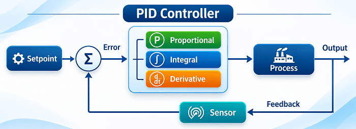
A PID controller diagram is a block diagram of a closed loop. The diagram shows the set point, error summation, PID controller, process, output and sensor to report back the value. This can be seen in the image below.
Set Point
This is the value you want. It can be entered manually on a display or via software. You can see a summing junction after a set point in the small circle. It compares the setpoint with the measured value and gives you the error. This is simple subtraction.
PID Controller
This is the main component. Here, the three terms are applied. The P term multiplies the error by a gain value. The I term adds up the error over time. The D term looks at how quickly the error is increasing/decreasing. These three values are then added together to create an output signal.
Process (Plant)
This is what you’re trying to control. This can be a heater and chamber, motor and load or valve and pipe. It will respond to the signal from the controller either slowly or quickly, depending on its nature.
Output
This is the actual value you’re interested in. For example, the temperature of the chamber.
Sensor
This measures the output. This could be a thermocouple, encoder or pressure transducer. This is an important part of the loop. If you don’t have a good sensor, then it is all guesswork.
PID Controller Working Principle
PID works on a closed loop feedback principle. The controller measures the output and calculates the error. The error is then corrected using the three terms. The PID controller will apply the proportional, integral & derivative terms to its signal to reduce the error as much as possible.
The general equation for PID control is: Output = (Kp x Error) + (Ki x Total error) + (Kd x Rate of change of error). Kp, Ki & Kd are gains that indicate how strong each term is.
The P term applies a quick burst of power in proportion to the error. If the error is high, more power is applied. This will, however, cause a small amount of error to remain as the P term will reduce as the error reduces. This can be corrected by the I term. The I term will continue to add to any remaining error until there is no error. This can cause problems if too much is applied as it will cause the system to overshoot.
The D term acts as a brake. It will notice the error is reducing quickly and will reduce the output slightly. If too much D is applied, it will cause the loop to become jittery especially if the sensor is noisy.
Overall, there needs to be a balance between the three terms. Tuning is the process of adjusting the gains. This is where most of the actual work is. Using methods like Ziegler-Nichols will give a starting point but most of the time you will need to fine-tune by observing the response.
How Does The PID Controller Work?
In practice, PID controllers constantly run a loop. The controller will take a reading from the sensor, calculate the error, apply the P, I & D terms and send out a new output. This will cause the process to move closer to the set point.
An example will help. Let’s say the oven is set to 100 degrees and the room is at 30 degrees.
Initially, the error will be large at 70. The P term will be high, causing the heater to increase to near max power and the temperature to rise quickly. The I term will be small.
As the temperature reaches around 80 degrees, the error will be reduced to 20. The heater will reduce its power. The D term will notice the temperature is rising quickly and will reduce the power slightly further to stop the oven from speeding past.
As the temperature gets close to 100 (around 98/99), the P term will cause the power to be very low. However, due to the I term adding a small amount of error, the output will increase slightly. The temperature will settle at 100 degrees.
If someone then opens the door, the temperature will drop to 94. The error will increase, resulting in the P term reacting immediately. The I term will continue to increase until the heat is regained. The D term will smooth the regain to stop it from overshooting. The loop will never fully stop.
PID control can be found in many places. For example, furnace/oven control, motor speed drives, robot arms, drones, chemical plants, HVAC systems and pressure/flow control. Any application where you need to keep a constant value will most likely have a PID hidden away.
Conclusion
PID control helps to keep a value constant by monitoring the error and correcting it using the current, past and forecasted data. Each term helps to overcome a weakness, making a stable and quick response. Once you understand how the set point, controller, process and sensor form a loop, most of the work is tuning.
At Testronix Instruments, we build laboratory testing equipment where exact thermal and environmental stability directly impacts your test results. For example, our Heat Seal Testers rely on dual PID controllers to hold upper & lower sealing jaws within fractions of a degree. Our Digital Humidity Chambers and Melt Flow Indexers use precision PID loops to lock in chamber climates and barrel temperatures during long test cycles. If you are looking for reliable testing equipment backed by accurate, well-tuned control loops, explore the full range at Testronix Instruments.